Note
Go to the end to download the full example code
Brightfield TFM & Cropped Input
This example calculates traction forces around an individual immune cell (NK92 natural killer cell) during migrtion in a collagen 1.2mg/ml networks (Batch C).
Here simple brightfield image stacks are used to calculate the matrix deformations & forces around the cell.
We compare the contracted state with the previous time step 30 seconds earlier. The cell of interest is cropped from a larger field of view.
This example can also be evaluated within the graphical user interface.
24 import saenopy
Loading the Stacks
Saenopy is very flexible in loading stacks from any filename structure. Here, we use only brightfield images without additional channels. We compare the stack in the contracted state with a reference state 30 seconds earlier. We load one multitiff file per stack, where each individual image corresponds to the [z] position. Experimentally, it can be convenient to take a larger field of view and crop it later to an area of interest. For this purpose, we use the “crop” parameter, which specifies the boundaries of region of intrest (in pixel). The “crop” parameter can be set both from the user interface and from the Python code.
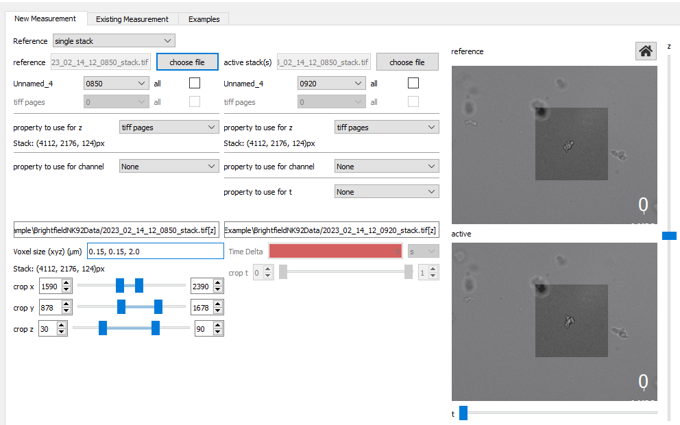
We load the relaxed and the contracted stack by using the placeholder [z] for the z stack in mutlitiffs
47 results = saenopy.get_stacks(
48     'BrightfieldNK92Data/2023_02_14_12_0920_stack.tif[z]',
49     reference_stack='BrightfieldNK92Data/2023_02_14_12_0850_stack.tif[z]',
50     output_path='BrightfieldNK92Data/example_output',
51     voxel_size=[0.15, 0.15, 2.0],
52     crop={'x': (1590, 2390), 'y': (878, 1678), 'z': (30, 90)},
53     )
Detecting the Deformations
Saenopy uses 3D Particle Image Velocimetry (PIV) with the following parameters to calculate matrix deformations between a deformed and relaxed state.
Piv Parameter |
Value |
|---|---|
element_size |
4.8 |
window_size |
12.0 |
signal_to_noise |
1.3 |
drift_correction |
True |
Small image features enable to measure 3D deformations from the brightfield stack
 87 # define the parameters for the piv deformation detection
 88 piv_parameters = {'element_size': 4.8, 'window_size': 12.0, 'signal_to_noise': 1.3, 'drift_correction': True}
 89
 90
 91 # iterate over all the results objects
 92 for result in results:
 93     # set the parameters
 94     result.piv_parameters = piv_parameters
 95     # get count
 96     count = len(result.stacks)
 97     if result.stack_reference is None:
 98         count -= 1
 99     # iterate over all stack pairs
100     for i in range(count):
101         # or two consecutive stacks
102         if result.stack_reference is None:
103             stack1, stack2 = result.stacks[i], result.stacks[i + 1]
104         # get both stacks, either reference stack and one from the list
105         else:
106             stack1, stack2 = result.stack_reference, result.stacks[i]
107         # and calculate the displacement between them
108         result.mesh_piv[i] = saenopy.get_displacements_from_stacks(stack1, stack2,
109                                                                    piv_parameters["window_size"],
110                                                                    piv_parameters["element_size"],
111                                                                    piv_parameters["signal_to_noise"],
112                                                                    piv_parameters["drift_correction"])
113     # save the displacements
114     result.save()
Generating the Finite Element Mesh
We interpolate the found deformations onto a new mesh which will be used for the regularisation. with the following parameters.
Mesh Parameter |
Value |
|---|---|
element_size |
4.0 |
mesh_size_same |
‘piv’ |
reference_stack |
‘next’ |
135 # define the parameters to generate the solver mesh and interpolate the piv mesh onto it
136 mesh_parameters = {'reference_stack': 'next', 'element_size': 4.0, 'mesh_size': 'piv'}
137
138 # iterate over all the results objects
139 for result in results:
140     # correct for the reference state
141     displacement_list = saenopy.subtract_reference_state(result.mesh_piv, mesh_parameters["reference_stack"])
142     # set the parameters
143     result.mesh_parameters = mesh_parameters
144     # iterate over all stack pairs
145     for i in range(len(result.mesh_piv)):
146         # and create the interpolated solver mesh
147         result.solvers[i] = saenopy.interpolate_mesh(result.mesh_piv[i], displacement_list[i], mesh_parameters)
148     # save the meshes
149     result.save()
Calculating the Forces
Define the material model and run the regularisation to fit the measured deformations and get the forces.
Material Parameter |
Value |
|---|---|
k |
6062 |
d_0 |
0.0025 |
lambda_s |
0.0804 |
d_s |
0.034 |
Regularisation Parameter |
Value |
|---|---|
alpha |
10**11 |
step_size |
0.33 |
max_iterations |
300 |
rel_conv_crit |
0.01 |
181 # define the parameters to generate the solver mesh and interpolate the piv mesh onto it
182 material_parameters = {'k': 6062.0, 'd_0': 0.0025, 'lambda_s': 0.0804, 'd_s':  0.034}
183 solve_parameters = {'alpha': 10**11, 'step_size': 0.33, 'max_iterations': 300, 'rel_conv_crit': 0.01}
184
185 # iterate over all the results objects
186 for result in results:
187     result.material_parameters = material_parameters
188     result.solve_parameters = solve_parameters
189     for index, M in enumerate(result.solvers):
190         # set the material model
191         M.set_material_model(saenopy.materials.SemiAffineFiberMaterial(
192             material_parameters["k"],
193             material_parameters["d_0"],
194             material_parameters["lambda_s"],
195             material_parameters["d_s"],
196         ))
197         # find the regularized force solution
198         M.solve_regularized(alpha=solve_parameters["alpha"], step_size=solve_parameters["step_size"],
199                             max_iterations=solve_parameters["max_iterations"],
200                             rel_conv_crit=solve_parameters["rel_conv_crit"], verbose=True)
201         # save the forces
202         result.save()
203         # clear the cache of the solver
204         results.clear_cache(index)
Display Results
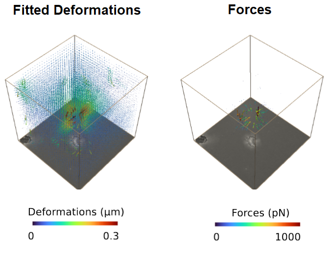
The reconstructed force field (right) generates a reconstructed deformation field (left) that recapitulates the measured matrix deformation field (upper video). The overall cell contractility is calculated as all force components pointing to the force epicenter.
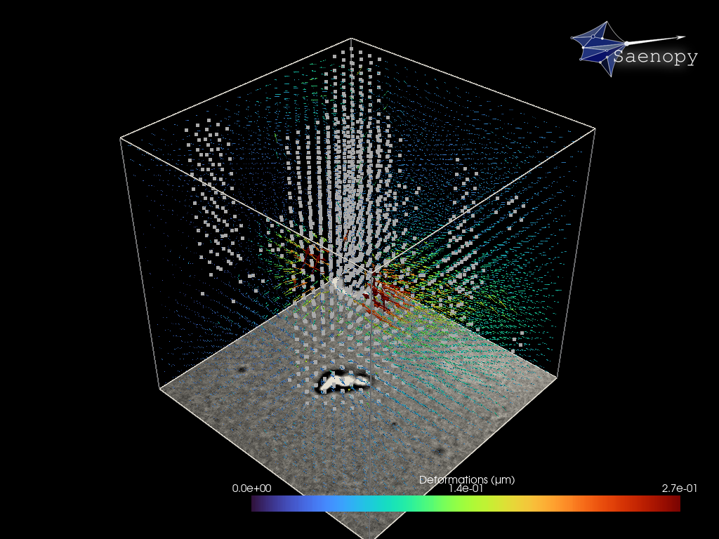
The cell occupied area is omitted since the signal to noise filter replaces the limited information with Nan values (Grey Dots). Therefore, no additional segmentation is required. Since we are working with simple brightfield images here, we do not have information below and above the cell.