Classic TFM (liver fibroblasts)

This example evaluates three hepatic stellate cells in 1.2mg/ml collagen with relaxed and deformed stacks. The relaxed stacks were recorded with cytochalasin D treatment of the cells. This example can also be evaluated with the graphical user interface.

import saenopy

Downloading the example data files

The folder structure is as follows. There are three cells recorded at different positions in the gel (Pos004, Pos007, Pos008) and three channels (ch00, ch01, ch02). The stack has 376 z positions (z000-z375). All positions are recorded once in the active state (“Deformed”) and once after relaxation with Cyto D as the reference state (“Relaxed”).

1_ClassicSingleCellTFM
├── Deformed
│   └── Mark_and_Find_001
│       ├── Pos004_S001_z000_ch00.tif
│       ├── Pos004_S001_z000_ch01.tif
│       ├── Pos004_S001_z000_ch02.tif
│       ├── Pos004_S001_z001_ch02.tif
│       ├── ...
│       ├── Pos007_S001_z001_ch00.tif
│       ├── ...
│       ├── Pos008_S001_z001_ch02.tif
│       └── ...
└── Relaxed
    └── Mark_and_Find_001
        ├── Pos004_S001_z000_ch00.tif
        ├── Pos004_S001_z000_ch01.tif
        ├── Pos004_S001_z000_ch02.tif
        ├── Pos004_S001_z001_ch02.tif
        ├── ...
        ├── Pos007_S001_z001_ch00.tif
        ├── ...
        ├── Pos008_S001_z001_ch02.tif
        └── ...

# download the data
saenopy.load_example("ClassicSingleCellTFM")

Loading the Stacks

Saenopy is very flexible in loading stacks from any filename structure. Here we replace the number in the position “Pos004” with an asterisk “Pos*” to batch process all positions. We replace the number of the channels “ch00” with a channel placeholder “ch{c:00}” to indicate that this refers to the channels and which channel to use as the first channel where the deformations should be detected. We replace the number of the z slice “z000” with a z placeholder “z{z}” to indicate that this number refers to the z slice. We do the same for the deformed state and for the reference stack.

# load the relaxed and the contracted stack
# {z} is the placeholder for the z stack
# {c} is the placeholder for the channels
# {t} is the placeholder for the time points
results = saenopy.get_stacks(
    '1_ClassicSingleCellTFM/Deformed/Mark_and_Find_001/Pos*_S001_z{z}_ch{c:00}.tif',
    reference_stack='1_ClassicSingleCellTFM/Relaxed/Mark_and_Find_001/Pos*_S001_z{z}_ch{c:00}.tif',
    output_path='1_ClassicSingleCellTFM/example_output',
    voxel_size=[0.7211, 0.7211, 0.988])

Detecting the Deformations

Saenopy uses 3D Particle Image Velocimetry (PIV) with the following parameters to calculate matrix deformations between a deformed and relaxed state for three example cells.

Piv Parameter	Value
element_size	14
window_size	35
signal_to_noise	1.3
drift_correction	True

# define the parameters for the piv deformation detection
piv_parameters = {'element_size': 14.0, 'window_size': 35.0, 'signal_to_noise': 1.3, 'drift_correction': True}

# iterate over all the results objects
for result in results:
    # set the parameters
    result.piv_parameters = piv_parameters
    # get count
    count = len(result.stacks)
    if result.stack_reference is None:
        count -= 1
    # iterate over all stack pairs
    for i in range(count):
        # get two consecutive stacks
        if result.stack_reference is None:
            stack1, stack2 = result.stacks[i], result.stacks[i + 1]
        # or reference stack and one from the list
        else:
            stack1, stack2 = result.stack_reference, result.stacks[i]
        # and calculate the displacement between them
        result.mesh_piv[i] = saenopy.get_displacements_from_stacks(stack1, stack2,
                                                                   piv_parameters["window_size"],
                                                                   piv_parameters["element_size"],
                                                                   piv_parameters["signal_to_noise"],
                                                                   piv_parameters["drift_correction"])
    # save the displacements
    result.save()

Generating the Finite Element Mesh

Interpolate the found deformations onto a new mesh which will be used for the regularisation. We use identical element size of deformation detection mesh here and keep the overall mesh size the same.

Mesh Parameter	Value
element_size	14
mesh_size	‘piv’
reference_stack	‘first’

# define the parameters to generate the solver mesh and interpolate the piv mesh onto it
mesh_parameters = {'reference_stack': 'first', 'element_size': 14.0, 'mesh_size': 'piv'}


# iterate over all the results objects
for result in results:
    # correct for the reference state
    displacement_list = saenopy.subtract_reference_state(result.mesh_piv, mesh_parameters["reference_stack"])
    # set the parameters
    result.mesh_parameters = mesh_parameters
    # iterate over all stack pairs
    for i in range(len(result.mesh_piv)):
        # and create the interpolated solver mesh
        result.solvers[i] = saenopy.interpolate_mesh(result.mesh_piv[i], displacement_list[i], mesh_parameters)
    # save the meshes
    result.save()

Calculating the Forces

Define the material model and run the regularisation to fit the measured deformations and get the forces.

Material Parameter	Value
k	6062
d_0	0.0025
lambda_s	0.0804
d_s	0.034

Regularisation Parameter	Value
alpha	10**10
step_size	0.33
max_iterations	400
rel_conv_crit	0.009

# define the parameters to generate the solver mesh and interpolate the piv mesh onto it
material_parameters = {'k': 6062.0, 'd_0': 0.0025, 'lambda_s': 0.0804, 'd_s':  0.03}
solve_parameters = {'alpha': 10**10, 'step_size': 0.33, 'max_iterations': 400, 'rel_conv_crit': 0.009}

# iterate over all the results objects
for result in results:
    result.material_parameters = material_parameters
    result.solve_parameters = solve_parameters
    for M in result.solvers:
        # set the material model
        M.set_material_model(saenopy.materials.SemiAffineFiberMaterial(
            material_parameters["k"],
            material_parameters["d_0"],
            material_parameters["lambda_s"],
            material_parameters["d_s"],
        ))
        # find the regularized force solution
        M.solve_regularized(alpha=solve_parameters["alpha"], step_size=solve_parameters["step_size"],
                            max_iterations=solve_parameters["max_iterations"],
                            rel_conv_crit=solve_parameters["rel_conv_crit"], verbose=True)
    # save the forces
    result.save()

Display Results

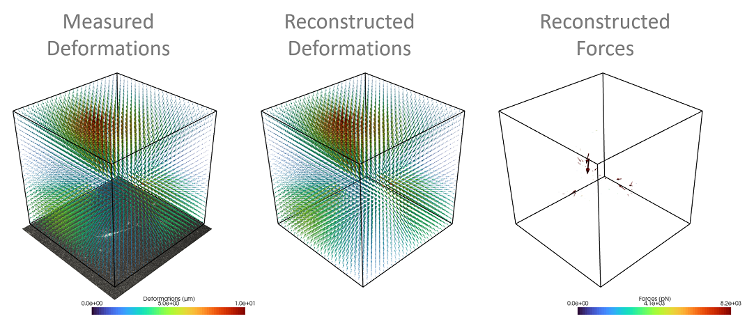
The reconstructed force field (right) generates a reconstructed deformation field (middle) that recapitulates the measured matrix deformation field (left). The overall cell contractility is calculated as all forcecomponents pointing to the force epicenter.