Material

The core of the saenopy package is its unique material model for fibered hydrogels, which is explained in the following section.

Semi-Affine Fibers

The stiffness \(\omega''(\lambda)\) as a function of the strain. It is the second derivative of the energy function \(\omega(\lambda)\) of the material, which is used for the calculation as explained below.

The default material model is a semi-affine fiber material which is approximated by a mean field description. Semi-affine because the model material is not an affine material, but nevertheless shows some affine properties. The mean field description means that not individual fibers are simulated but the mean effect of them, as described below.

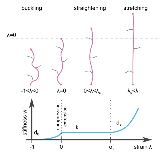
The fibers are modeled to show different behavior in three strain regimes:

• under compression (\(-1 < \lambda < 0\)) fibers buckle showing an exponential decay of the stiffness

• for small strains (\(0<\lambda<\lambda_s\)) fibers show a linear stiffness

• for larger strains (\(\lambda_s<\lambda\)) fibers show strain stiffening with an exponential increase of the stiffness

\[\begin{split}w''(\lambda) = \begin{cases} k \exp\left(\frac{\lambda}{d_0}\right) &\mbox{if } -1 \le \lambda < 0 & \mbox{buckling} \\ k & \mbox{if } 0 \le \lambda < \lambda_s & \mbox{linear} \\ k \exp\left(\frac{\lambda-\lambda_s}{d_s}\right) &\mbox{if } \lambda_s \le \lambda & \mbox{stiffening} \\ \end{cases}\end{split}\]

With the stiffness \(k\), the buckling exponent \(d_0\), the stiffening threshold \(\lambda_s\) and the stiffening exponent \(d_s\).

The energy function \(w(\lambda)\) is then used to calculate the energy stored in a tetrahedron with a deformation gradient \(\mathbf{F}\), by applying the deformation gradient to a finite set of homogeneously distributed unit vectors \(\vec{e_r}(\Omega)\). The strain \(\lambda\) of these vectors is used to calculate the energy \(w\) stored in this deformation. The energy density \(W\) is the average of the contributions of all these unit vectors \(\vec{e_r}(\Omega)\); resulting in an average (mean field approach) of the energy over the full solid angle, assuming that possible fibers are distributed isotropically.

\[W = \langle\omega(|\mathbf{F} \cdot \vec{e_r}(\Omega)|-1)\rangle_\Omega\]

With \(\mathbf{F}\) being the deformation gradient, \(\vec{e_r}\) a unit vector in a finite set of directions that approximate \(\Omega\) the solid angle, \(\omega(\lambda)\) the material’s energy function, \(W\) the energy density and \(\langle \cdot \rangle_\Omega\) denotes an average over the solid angle.

Materials

This section documents the class that represents this material.

class saenopy.materials.Material

The base class for all material models.

class saenopy.materials.SemiAffineFiberMaterial(k, d_0=None, lambda_s=None, d_s=None)

This class defines the default material of saenopy. The fibers show buckling (i.e. decaying stiffness) for -1 < lambda < 0, a linear stiffness response for small strains 0 < lambda < lambda_s, and strain stiffening for large strains lambda_s < lambda.

Parameters:

• k (float) – The stiffness of the material in the linear regime.

• d_0 (float, optional) – The decay parameter in the buckling regime. If omitted the material shows no buckling but has a linear response for compression.

• lambda_s (float, optional) – The stretching where the strain stiffening starts. If omitted the material shows no strain stiffening.

• d_s (float, optional) – The parameter specifying how strong the strain stiffening is. If omitted the material shows no strain stiffening.

Defining custom materials

To define a custom material, define a new class that is a subclass of saenopy.materials.Material. The class needs to define a function called stiffness to define the material model. Saenopy will call this function with an array of stretch values and the function has to an array of the corresponding stiffness values.

This procedure is demonstrated in the following code example where a new material QuadracticMaterial is defined with a stiffness function that is linearly dependent on the stretch, i.e. resulting in a quadratic force response.

from saenopy.materials import Material

class QuadracticMaterial(Material):
    """
    A custom material that has a quadratic force response.

    Parameters
    ----------
    k : float
        The stiffness of the material.
    """
    def __init__(self, k):
        # parameters
        self.k = k
        self.parameters = dict(k=k)

    def stiffness(self, s):
        # the stiffness increases linearly, resulting in a quadratic force
        stiff = self.k * s

        return stiff

The newly defined material can be used with setMaterialModel().

Macrorheology

As the material model is based on microscopic parameters and not on macroscopic parameters (as e.g. the bulk stiffness), the material parameters cannot directly be measured using a rheometer. Instead the rheological experiments are “simulated” on the material model and the resulting curves can be used to fit the material parameters so that the the “simulated” rheological experiments on the material model fit the measured rheological response of the material.

Here, we describe three different rheological experiments that can be simulated on the material model.

• Shear Rheometer

• Stretch Thinning

• Extensional Rheometer

The stretch experiment is needed to reliably fit later on the buckling of the material and either the Shear Rheometer or the Extensional Rheometer experiment can be used to fit the fiber stiffness and the strain stiffening.

This section first describes the functions that simulate these experiments on the material model and the next section explains how these functions can be used to fit the material parameters from experimental data.

Shear Rheometer

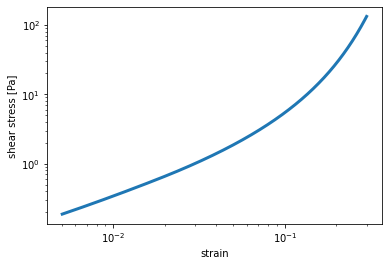
saenopy.macro.get_shear_rheometer_stress(gamma: ~numpy.ndarray, material: ~saenopy.materials.Material, s: ~numpy.ndarray | None = None) -> (<class 'numpy.ndarray'>, <class 'numpy.ndarray'>)

This function returns the stress the material model generates when subjected to a shear strain, as seen in a shear rheometer.

The shear strain is described using the following deformation gradient \(\mathbf{F}\):

\[\begin{split}\mathbf{F}(\gamma) = \begin{pmatrix} 1 & \gamma & 0 \\ 0 & 1 & 0 \\ 0 & 0 & 1 \\ \end{pmatrix}\end{split}\]

and the resulting stress is obtained by calculating numerically the derivative of the energy density \(W\) with respect to the strain \(\gamma\):

\[\sigma(\gamma) = \frac{dW(\mathbf{F}(\gamma))}{d\gamma}\]

Parameters:

• gamma (ndarray) – The strain values for which to calculate the stress.

• material (Material) – The material model to use.

Returns:

• strain (ndarray) – The strain values.

• stress (ndarray) – The resulting stress.

%matplotlib inline

import numpy as np
import matplotlib.pyplot as plt

from saenopy import macro
from saenopy.materials import SemiAffineFiberMaterial

material = SemiAffineFiberMaterial(900, 0.0004, 0.0075, 0.033)
print(material)

gamma = np.arange(0.005, 0.3, 0.0001)
x, y = macro.get_shear_rheometer_stress(gamma, material)
plt.loglog(x, y, "-", lw=3, label="model")

plt.xlabel("strain")
plt.ylabel("shear stress [Pa]")

plt.show()

SemiAffineFiberMaterial(k=900, d0=0.0004, lambda_s=0.0075, ds=0.033)

Stretcher

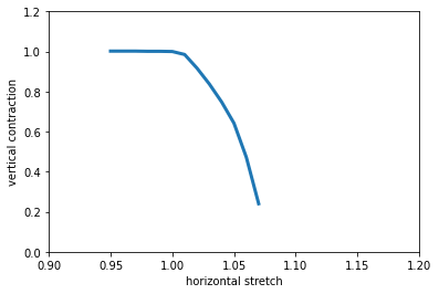
saenopy.macro.get_stretch_thinning(gamma_h, gamma_v, material, s=None)

This function returns the vertical thinning (strain in z direction) of the material model when the material model is stretched horizontally (strain in x direction), as seen in a stretcher device.

The strain in x and z direction is described using the following deformation gradient \(\mathbf{F}\):

\[\begin{split}\mathbf{F}(\gamma) = \begin{pmatrix} \gamma_h & 0 & 0 \\ 0 & 1 & 0 \\ 0 & 0 & \gamma_v \\ \end{pmatrix}\end{split}\]

the resulting energy density \(W(\mathbf{F}(\gamma_h,\gamma_v))\) is then minimized numerically for every \(\gamma_h\) to obtain the \(\gamma_v\) that results in the lowest energy of the system.

Parameters:

• gamma_h (ndarray) – The applied strain in horizontal direction.

• gamma_v (ndarray) – The different values for thinning to test. The value with the lowest energy for each horizontal strain is returned.

• material (Material) – The material model to use.

Returns:

• gamma_h (ndarray) – The horizontal strain values.

• gamma_v (ndarray) – The vertical strain that minimizes the energy for the horizontal strain.

import numpy as np
import matplotlib.pyplot as plt

from saenopy import macro
from saenopy.materials import SemiAffineFiberMaterial

material = SemiAffineFiberMaterial(900, 0.0004, 0.0075, 0.033)
print(material)

lambda_h = np.arange(1-0.05, 1+0.07, 0.01)
lambda_v = np.arange(0, 1.1, 0.001)

x, y = macro.get_stretch_thinning(lambda_h, lambda_v, material)
plt.plot(x, y, lw=3, label="model")
plt.xlabel("horizontal stretch")
plt.ylabel("vertical contraction")

plt.ylim(0, 1.2)
plt.xlim(0.9, 1.2)

plt.show()

SemiAffineFiberMaterial(k=900, d0=0.0004, lambda_s=0.0075, ds=0.033)

Extensional Rheometer

saenopy.macro.get_extensional_rheometer_stress(gamma, material, s=None)

This function returns the stress the material model generates when subjected to an extensional strain, as seen in an extensional rheometer.

The extensional strain is described using the following deformation gradient \(\mathbf{F}\):

\[\begin{split}\mathbf{F}(\gamma) = \begin{pmatrix} \gamma & 0 & 0 \\ 0 & 1 & 0 \\ 0 & 0 & 1 \\ \end{pmatrix}\end{split}\]

and the resulting stress is obtained by calculating numerically the derivative of the energy density \(W\) with respect to the strain \(\gamma\):

\[\sigma(\gamma) = \frac{dW(\mathbf{F}(\gamma))}{d\gamma}\]

Parameters:

• gamma (ndarray) – The strain values for which to calculate the stress.

• material (Material) – The material model to use.

Returns:

• strain (ndarray) – The strain values.

• stress (ndarray) – The resulting stress.

import numpy as np
import matplotlib.pyplot as plt

from saenopy import macro
from saenopy.materials import SemiAffineFiberMaterial, LinearMaterial

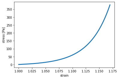
material = SemiAffineFiberMaterial(900, 0.0004, 0.0075, 0.033)
print(material)

epsilon = np.arange(1, 1.17, 0.0001)
x, y = macro.get_extensional_rheometer_stress(epsilon, material)
plt.plot(x, y, lw=3, label="model")

plt.xlabel("strain")
plt.ylabel("stress [Pa]")

plt.show()

SemiAffineFiberMaterial(k=900, d0=0.0004, lambda_s=0.0075, ds=0.033)

Fitting material parameters

To fit the parameters of the material model for the use withe saenopy four parameters are needed, as explained above.

from saenopy import macro
import numpy as np

# example data, stress-strain curves for collagen of three different concentrations
data0_6 = np.array([[4.27e-06,-2.26e-03],[1.89e-02,5.90e-01],[3.93e-02,1.08e+00],[5.97e-02,1.57e+00],[8.01e-02,2.14e+00],[1.00e-01,2.89e+00],[1.21e-01,3.83e+00],[1.41e-01,5.09e+00],[1.62e-01,6.77e+00],[1.82e-01,8.94e+00],[2.02e-01,1.17e+01],[2.23e-01,1.49e+01],[2.43e-01,1.86e+01],[2.63e-01,2.28e+01],[2.84e-01,2.71e+01]])
data1_2 = np.array([[1.22e-05,-1.61e-01],[1.71e-02,2.57e+00],[3.81e-02,4.69e+00],[5.87e-02,6.34e+00],[7.92e-02,7.93e+00],[9.96e-02,9.56e+00],[1.20e-01,1.14e+01],[1.40e-01,1.35e+01],[1.61e-01,1.62e+01],[1.81e-01,1.97e+01],[2.02e-01,2.41e+01],[2.22e-01,2.95e+01],[2.42e-01,3.63e+01],[2.63e-01,4.43e+01],[2.83e-01,5.36e+01],[3.04e-01,6.37e+01],[3.24e-01,7.47e+01],[3.44e-01,8.61e+01],[3.65e-01,9.75e+01],[3.85e-01,1.10e+02],[4.06e-01,1.22e+02],[4.26e-01,1.33e+02]])
data2_4 = np.array([[2.02e-05,-6.50e-02],[1.59e-02,8.46e+00],[3.76e-02,1.68e+01],[5.82e-02,2.43e+01],[7.86e-02,3.34e+01],[9.90e-02,4.54e+01],[1.19e-01,6.11e+01],[1.40e-01,8.16e+01],[1.60e-01,1.06e+02],[1.80e-01,1.34e+02],[2.01e-01,1.65e+02],[2.21e-01,1.96e+02],[2.41e-01,2.26e+02]])

# hold the buckling parameter constant, as it cannot be determined well with shear experiments
d_s0 = 0.003
# minimize 3 shear rheometer experiments with different collagen concentration and, therefore, different k1 parameters
# but keep the other parameters the same
parameters, plot = macro.minimize([
        [macro.get_shear_rheometer_stress, data0_6, lambda p: (p[0], d_s0, p[3], p[4])],
        [macro.get_shear_rheometer_stress, data1_2, lambda p: (p[1], d_s0, p[3], p[4])],
        [macro.get_shear_rheometer_stress, data2_4, lambda p: (p[2], d_s0, p[3], p[4])],
    ],
    [900, 1800, 12000, 0.03, 0.08],
)



# print the resulting parameters
print(parameters)
# and plot the results
plot()

u:\dropbox\software-github\saenopy\real\saenopy\macro.py:469: RuntimeWarning: invalid value encountered in log
  cost = np.nansum((np.log(stretchy2) - np.log(sheary)) ** 2 * weights)

[6.81340555e+02 2.92017024e+03 1.10147721e+04 2.93635523e-02
 8.06826765e-02]

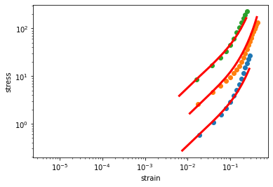
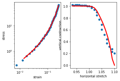
To fit all parameters, experiments of different types should be combined, e.g. a shear rheological experiment and a stretching experiment.

from saenopy import macro
import numpy as np

# example data, stress-strain curves and a stretch experiment
shear = np.array([[7.50e-03,2.78e-01],[1.25e-02,4.35e-01],[1.75e-02,6.44e-01],[2.25e-02,7.86e-01],[2.75e-02,9.98e-01],[3.25e-02,1.13e+00],[3.75e-02,1.52e+00],[4.25e-02,1.57e+00],[4.75e-02,1.89e+00],[5.25e-02,2.10e+00],[5.75e-02,2.46e+00],[6.25e-02,2.67e+00],[6.75e-02,3.15e+00],[7.25e-02,3.13e+00],[7.75e-02,3.83e+00],[8.25e-02,4.32e+00],[8.75e-02,4.35e+00],[9.25e-02,4.78e+00],[9.75e-02,5.45e+00],[1.02e-01,5.87e+00],[1.07e-01,6.16e+00],[1.13e-01,6.89e+00],[1.17e-01,7.89e+00],[1.22e-01,8.28e+00],[1.28e-01,9.13e+00],[1.33e-01,1.06e+01],[1.38e-01,1.10e+01],[1.42e-01,1.27e+01],[1.47e-01,1.39e+01],[1.52e-01,1.53e+01],[1.58e-01,1.62e+01],[1.63e-01,1.78e+01],[1.68e-01,1.89e+01],[1.72e-01,2.03e+01],[1.77e-01,2.13e+01],[1.82e-01,2.23e+01],[1.88e-01,2.38e+01],[1.93e-01,2.56e+01],[1.98e-01,2.78e+01],[2.03e-01,3.02e+01],[2.07e-01,3.28e+01],[2.12e-01,3.55e+01],[2.17e-01,3.83e+01],[2.23e-01,4.13e+01],[2.28e-01,4.48e+01],[2.33e-01,4.86e+01],[2.37e-01,5.27e+01],[2.42e-01,5.64e+01],[2.47e-01,6.08e+01],[2.53e-01,6.48e+01],[2.58e-01,6.93e+01],[2.63e-01,7.44e+01],[2.68e-01,7.89e+01],[2.73e-01,8.40e+01],[2.78e-01,8.91e+01],[2.82e-01,9.41e+01],[2.87e-01,1.01e+02],[2.92e-01,1.07e+02],[2.97e-01,1.12e+02],[3.02e-01,1.19e+02],[3.07e-01,1.25e+02],[3.12e-01,1.32e+02],[3.18e-01,1.39e+02],[3.23e-01,1.45e+02],[3.28e-01,1.53e+02],[3.33e-01,1.60e+02],[3.38e-01,1.67e+02],[3.43e-01,1.76e+02],[3.47e-01,1.83e+02],[3.52e-01,1.90e+02],[3.57e-01,1.99e+02],[3.62e-01,2.06e+02],[3.67e-01,2.15e+02],[3.72e-01,2.23e+02],[3.78e-01,2.31e+02],[3.83e-01,2.40e+02],[3.88e-01,2.48e+02],[3.93e-01,2.56e+02],[3.98e-01,2.56e+02],[4.03e-01,2.73e+02],[4.07e-01,2.77e+02],[4.12e-01,2.86e+02],[4.17e-01,2.97e+02],[4.22e-01,3.08e+02],[4.27e-01,3.15e+02],[4.32e-01,3.25e+02],[4.38e-01,3.33e+02],[4.43e-01,3.39e+02],[4.48e-01,3.51e+02],[4.53e-01,3.59e+02],[4.58e-01,3.69e+02],[4.63e-01,3.76e+02],[4.68e-01,3.83e+02],[4.72e-01,3.93e+02],[4.77e-01,3.97e+02],[4.82e-01,4.04e+02],[4.87e-01,4.13e+02],[4.92e-01,4.18e+02],[4.97e-01,4.31e+02],[5.02e-01,4.38e+02],[5.07e-01,4.25e+02],[5.12e-01,4.48e+02],[5.17e-01,4.49e+02],[5.22e-01,4.56e+02],[5.27e-01,4.66e+02],[5.32e-01,4.70e+02],[5.37e-01,4.76e+02],[5.42e-01,4.82e+02],[5.47e-01,4.89e+02],[5.52e-01,4.99e+02],[5.57e-01,5.01e+02],[5.62e-01,5.06e+02],[5.68e-01,5.14e+02],[5.73e-01,5.15e+02],[5.78e-01,5.21e+02],[5.83e-01,5.28e+02],[5.88e-01,5.30e+02],[5.93e-01,5.38e+02],[5.98e-01,5.40e+02],[6.03e-01,5.41e+02],[6.08e-01,5.38e+02],[6.13e-01,5.39e+02],[6.18e-01,5.50e+02],[6.23e-01,5.56e+02],[6.27e-01,5.59e+02],[6.32e-01,5.68e+02],[6.37e-01,5.69e+02],[6.42e-01,5.70e+02],[6.47e-01,5.79e+02],[6.52e-01,5.78e+02],[6.57e-01,5.80e+02],[6.62e-01,5.83e+02],[6.67e-01,5.83e+02],[6.72e-01,5.89e+02],[6.77e-01,5.86e+02],[6.82e-01,5.88e+02],[6.88e-01,5.91e+02],[6.93e-01,5.86e+02],[6.98e-01,5.91e+02],[7.03e-01,5.91e+02],[7.08e-01,5.87e+02],[7.13e-01,5.89e+02],[7.18e-01,5.88e+02],[7.23e-01,5.89e+02],[7.28e-01,5.89e+02],[7.33e-01,5.81e+02],[7.38e-01,5.85e+02],[7.43e-01,5.86e+02],[7.48e-01,5.78e+02],[7.52e-01,5.78e+02],[7.57e-01,5.79e+02],[7.62e-01,5.76e+02],[7.67e-01,5.74e+02],[7.72e-01,5.70e+02],[7.77e-01,5.73e+02],[7.82e-01,5.70e+02],[7.87e-01,5.66e+02],[7.92e-01,5.69e+02],[7.97e-01,5.59e+02],[8.02e-01,5.50e+02],[8.07e-01,5.52e+02],[8.12e-01,5.52e+02],[8.18e-01,5.59e+02],[8.23e-01,5.58e+02],[8.28e-01,5.57e+02],[8.33e-01,5.59e+02],[8.38e-01,5.53e+02],[8.43e-01,5.55e+02],[8.48e-01,5.56e+02],[8.53e-01,5.49e+02],[8.58e-01,5.50e+02],[8.63e-01,5.47e+02],[8.68e-01,5.22e+02],[8.73e-01,5.44e+02],[8.77e-01,5.36e+02],[8.82e-01,5.38e+02],[8.87e-01,5.33e+02],[8.92e-01,5.28e+02],[8.97e-01,5.30e+02],[9.02e-01,5.23e+02],[9.07e-01,5.22e+02],[9.12e-01,5.18e+02],[9.17e-01,5.12e+02],[9.22e-01,5.11e+02],[9.27e-01,5.05e+02],[9.32e-01,5.03e+02],[9.38e-01,4.99e+02],[9.43e-01,4.88e+02],[9.48e-01,4.86e+02],[9.53e-01,4.82e+02],[9.58e-01,4.73e+02],[9.63e-01,4.70e+02],[9.68e-01,4.61e+02],[9.73e-01,4.56e+02],[9.78e-01,4.51e+02],[9.83e-01,4.41e+02],[9.88e-01,4.36e+02],[9.93e-01,4.22e+02],[9.98e-01,4.09e+02],[1.00e+00,4.07e+02]])[:50]
stretch = np.array([[9.33e-01,1.02e+00],[9.40e-01,1.01e+00],[9.47e-01,1.02e+00],[9.53e-01,1.02e+00],[9.60e-01,1.02e+00],[9.67e-01,1.01e+00],[9.73e-01,1.01e+00],[9.80e-01,1.01e+00],[9.87e-01,1.01e+00],[9.93e-01,1.00e+00],[1.00e+00,1.00e+00],[1.01e+00,9.89e-01],[1.01e+00,9.70e-01],[1.02e+00,9.41e-01],[1.03e+00,9.00e-01],[1.03e+00,8.46e-01],[1.04e+00,7.76e-01],[1.05e+00,6.89e-01],[1.05e+00,6.02e-01],[1.06e+00,5.17e-01],[1.07e+00,4.39e-01],[1.07e+00,3.74e-01],[1.08e+00,3.17e-01],[1.09e+00,2.72e-01],[1.09e+00,2.30e-01],[1.10e+00,2.02e-01]])

# fit all 4 parameters simultaneously to two experiments
parameters, plot = macro.minimize([
        [macro.get_shear_rheometer_stress, shear, lambda p: (p[0], p[1], p[2], p[3])],
        [macro.get_stretch_thinning, stretch, lambda p: (p[0], p[1], p[2], p[3])],
    ],
    [900, 0.0004, 0.075, 0.33],
)

# print the resulting parameters
print(parameters)
# and plot the results
plot()

[9.01527313e+02 9.67595545e-04 6.00863532e-03 3.28366376e-02]